Note: this was originally published on the UW-Hydro Blog.
Last month, we released VIC 5.0.0, a major rewrite of the user interface to and the infrastructure of the VIC model. We introduced this release in a recent blog post. This rewrite included a number of upgrades that will allow VIC to perform much better in high-performance computing (HPC) environments. In this blog post, I will discuss some of these improvements and illustrate how they may facilitate VIC applications at scales that were previously computationally infeasible.
Background
VIC was originally intended to be used as a land surface scheme (LSS) in general circulation models (GCMs) (Liang et al., 1994). However, the original source code was written as a stand-alone column model. In this configuration, distributed simulations were run one grid cell at a time, where the model would complete a simulation for a single grid cell for all timesteps prior to moving on to the next grid cell. We call this configuration “time-before-space”. From an infrastructure perspective, this meant VIC did not need built-in tools for parallelization or memory management for distributed simulations. Large scale (e.g. regional or global), distributed simulations were made possible through what we refer to as “poor man’s parallelization” where each grid cell was simulated as a separate task (even on a separate computer). For the past 15 years, this parallelization strategy has been sufficient for many VIC applications.
The development of VIC 5 was largely motivated by a number of limitations that were related to the legacy configuration of the VIC source code. First, despite this being one of VIC’s original goals, the “time-before-space” loop order precluded VIC’s direct coupling within GCMs, which typically require a “space-before-time” evaluation order. Second, VIC’s input/output (I/O) was designed to work with its “time-before-space” configuration. This meant there were individual forcing and output files for each grid cells. For large model domains, such as the Livneh et al. (2015) domain which included more than 330,000 grid cells, the sheer number of files that VIC users were having to deal with began to be the most challenging part of working with VIC. It also precluded the use of standard tools (such as ncview, cdo, xarray and others) that are designed to visualize and analyze large data sets. Not being able to visualize model output easily hampers model application and development. Third, a number of important hydrologic problems require a “space-before-time” configuration. For example, if upstream flow needs to be taken into account for local water and energy balance calculations, then it is necessary to perform routing after each model timestep. Routing requires information about the entire domain. While there are ways to accommodate this with prior VIC versions, these implementations tend to be awkward and aim to circumvent the “time-before-space” configuration. Implementation of a true “space-before-time” mode simplifies the integration of routing with the rest of the VIC model.
VIC 5 Developments for HPC
The largest change introduced in VIC 5 is the notion of individual drivers that all call the same physics routines. Because VIC has such as large user community and there are many ongoing projects that will use the legacy “time-before-space” configuration, we provided a classic driver, which essentially functions the same way as previous VIC implementations. For the reasons described above, most of our work on VIC 5 was focused on the development of a “space-before-time” configuration. We’re calling this the image driver.
The image driver has two main infrastructure improvements relative to the classic driver. First, we’ve incorporated a formal HPC parallelization strategy in the form of a Message Passing Interface (MPI). MPI is a standardized communication protocol for large parallel applications (out-of-core and off-node). In the context of VIC, it allows for the simultaneous simulation of thousands of grid-cells, distributed across a cluster or super-computer. Second, we’ve overhauled and standardized VIC’s I/O. Whereas previous versions of VIC used custom ASCII or binary file types, the image driver uses netCDF for both input and output files. NetCDF has been widely adopted throughout the geoscience community and offers three main advantages: first, it stores for N-dimensional binary datasets; second, it provides a standardized method for storing metadata along with the data; and third, there are many tools for visualizing and analyzing NetCDF files.
Scaling VIC on HPC
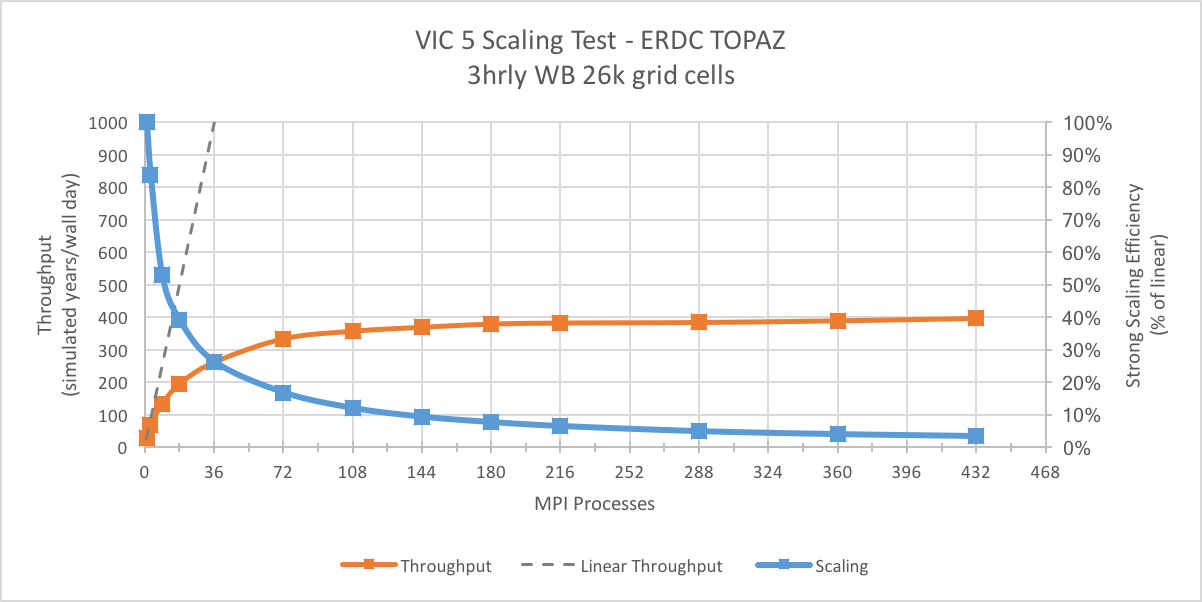
In this section, we will show an example of how VIC can be applied in parallel on a large super-computer. We’re showing results from two 1-year test simulations run using the image driver on the RASM model domain. The RASM model domain has about 26,000 land grid cells and includes the the entire pan-Arctic drainage. Both of these simulations were run using 3-hourly forcing inputs, a 3-hour model timestep, frozen soils, and minimal output (only 8 variables written once monthly). We ran these tests on the Topaz super-computer at the U.S. Department of Defense Engineer Research and Development Center Supercomputing Resource Center (ERDC DSRC). Topaz is a 124,416 core SGI ICE X machine, made up of 3,456 nodes (36 cores/node) capable 4.62 PFLOPS.
The first simulation we’re going to look at was run in “Water Balance” mode (FULL_ENERGY = FALSE).
When VIC is run in this mode it doesn’t iterate to find the surface temperature, resulting in much faster run times at the expense of model complexity.
The figure below shows the model throughput (left axis) for 15 identical VIC simulations run using between 1 and 432 MPI processes.
Using just 1 processor (no MPI), this VIC configuration has a model throughput of 27 model-years/wall-day (where one wall-day short for “wall-clock day” which is simply a calendar day in real time).
Using 72 processors, we see the model throughput increase 334 years/wall-day.
Beyond 36 processors, the throughput begins to plateau and the scaling efficiency (right axis) is too low to push the scaling any further.
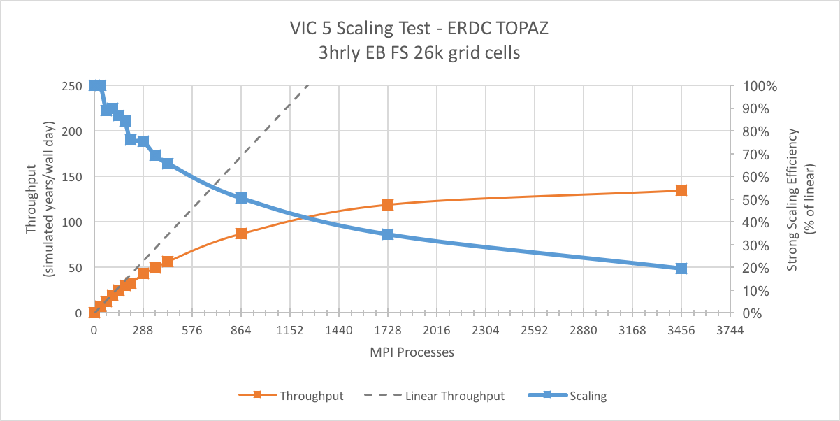
Next we’ll look at the scaling performance of VIC run in “Energy Balance” mode (FULL_ENERGY = TRUE).
When run in this configuration, we expect the model to be much more expensive.
In fact, we find that at 36 cores (one node), the throughput in the “Energy Balance” simulation is about 36 times less than the “Water Balance” simulation.
Because this configuration is so much more expensive, the scaling efficiency is substantially better.
In this case, the model throughput doesn’t really plateau after 864 processors where we’re able to get a throughput of 97 model-years/wall-day.
Conclusions
Our initial analysis of the VIC scaling shows us that for complex model configurations, we get reasonable scaling. With the scaling we’re seeing here, we can conceivably run 1000 year spinup simulations of VIC in the Arctic in 2-3 weeks. Another way to think about the potential here is in terms of applying VIC in large ensembles where 100s of ensemble members are run and readily analyzed using tools optimized for use with netCDF output. For simple VIC configurations (e.g. “Water Balance” only), it seems that VIC is not going to scale much beyond a single node, but it still benefits from multiple cores on the same node. The reason for this difference in scaling behavior lies in the interplay between the digital volume of input forcings (read on the master MPI processor and scattered to the slave processors) and computation performed on slave processors. As the input volume goes up or the computation time spent by individual slave processors goes down, the scaling performance decreases.
We are developing tools that automate these scaling tests. We also have a number of issues slated for future development that we believe will improve the scaling of VIC. The issues we think hold the most potential would add parallel netCDF I/O and on-node shared memory threading. Both of these features would reduce the overhead introduced by MPI.
Acknowledgments
Supercomputing resources were provided through the Department of Defense (DOD) High Performance Computing Modernization Program at the Army Engineer Research. Tony Craig, a member of the RASM team, also contributed to development of this blog.
References
- Liang, X., D. P. Lettenmaier, E. F. Wood, and S. J. Burges (1994), A simple hydrologically based model of land surface water and energy fluxes for general circulation models, J. Geophys. Res., 99(D7), 14415–14428, doi:10.1029/94JD00483.
- Livneh, B., Bohn, T.J., Pierce, D.W., Munoz-Arriola, F., Nijssen, B., Vose, R., Cayan, D.R. and Brekke, L., 2015. A spatially comprehensive, hydrometeorological data set for Mexico, the US, and Southern Canada 1950–2013. Scientific data, 2, doi:10.1038/sdata.2015.42.